Continuous Variation: Skills (DP IB Biology: SL): Revision Note
Written by: Emma Archbold
Updated on
Continuous Variation
Variation can be discrete or continuous
Discrete variation is variation that falls into two or more clear-cut categories with no overlap or in-between categories
Blood group is an example of discrete variation
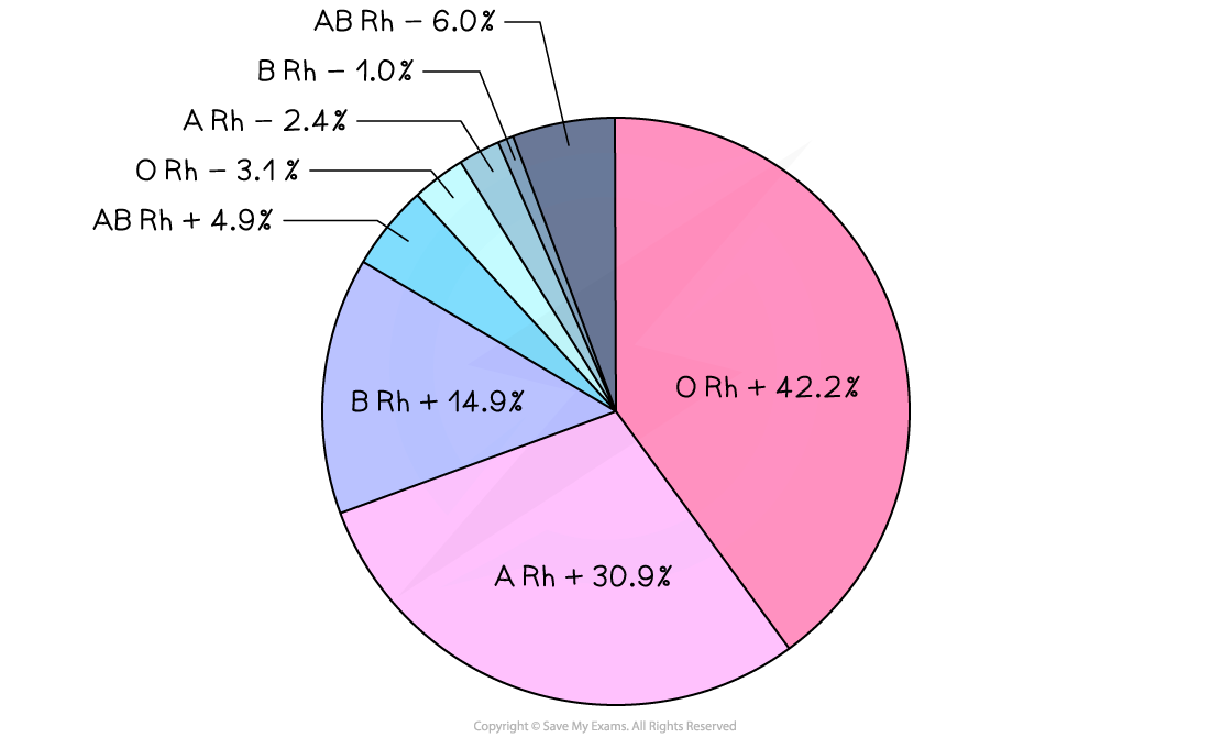
All human blood is either group O, A, B or AB, each with a Rhesus factor (+ or -)
This gives just 8 distinct blood groups:
Pie chart showing global blood group distribution

Worldwide A, B, O blood group distribution by percentage, 2019
(data varies regionally with ethnicity)
Continuous Variation
Continuous variation occurs when two or more genes affect the final characteristic
For example, height in humans is determined by many genetic factors:
Bone length
Skeletal muscle structure
Ability to absorb food substances effectively
Hormone production
…As well as environmental factors like diet, exercise, prenatal nutrition, lifestyle etc
Most characteristics are determined by more than one gene - a polygenic characteristic
Even grouped data like shoe size appears to be discrete but in fact, peoples' feet vary continuously in size
Shoe size is merely a practicality for shoe manufacturers, who cannot make exactly the right-sized shoes for everybody
Continuous variation in birth mass results in the population displaying a normal distribution (bell-shaped curve)
Environmental factors can also affect birth mass, e.g. mother's diet, presence of a twin, smoking etc
Continuous variation occurs when there are quantitative differences in the phenotypes of individuals within a population for particular characteristics
Quantitative differences do not fall into discrete categories like in discontinuous variation
For example, the mass or height of a human is an example of continuous variation
Instead for these features, a range of values exist between two extremes within which the phenotype will fall
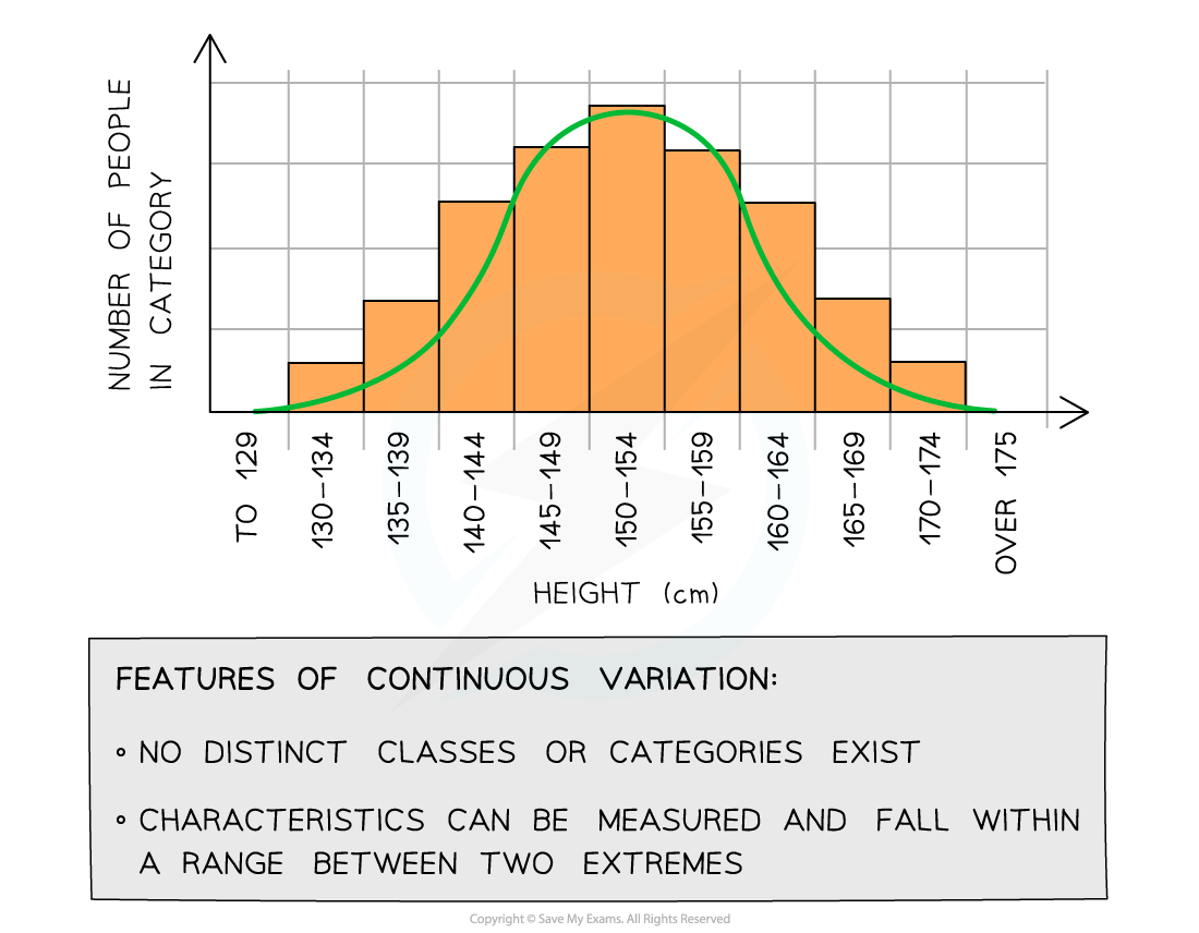
The lack of categories and the presence of a range of values can be used to identify continuous variation when it is presented in a table or graph
Normal distribution curve

Graph showing population variation in height: an example of continuous variation with quantitative differences
Genetic basis of continuous variation
This type of variation is caused by an interaction between genetics and the environment
Phenotype = genotype + environment
At the genetic level:
Different alleles at a single locus have a small effect on the phenotype
Different genes can have the same effect on the phenotype and these add together to have an additive effect
If a large number of genes have a combined effect on the phenotype they are known as polygenes
An example of a continuous polygenic trait is skin colour
Skin colour is determined by several genes that cause the production of a protein called melanin
The more melanin is produced, the darker the skin pigmentation becomes
Skin colour is also influenced by environmental factors such as UV exposure, which can cause the skin colour to become darker
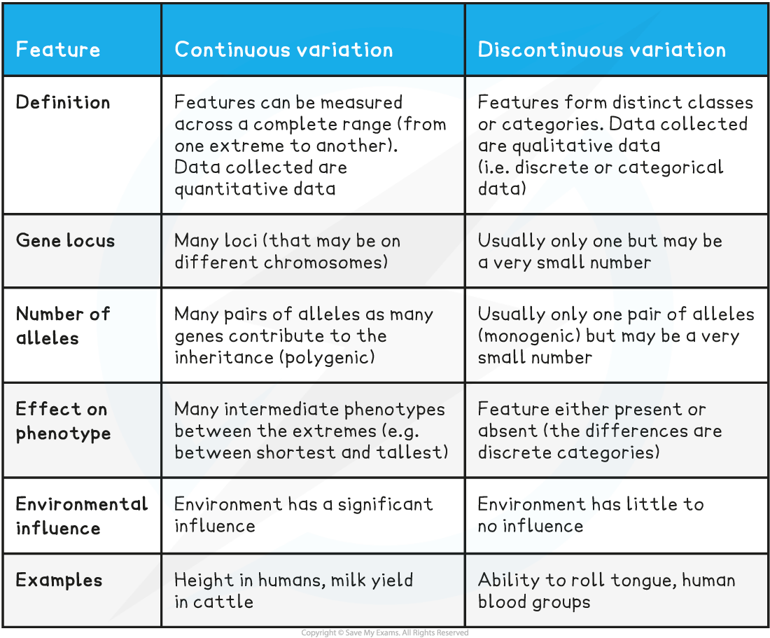
Comparison of Continuous and Discontinuous Variation Table

Box & Whisker Plots
What are box plots and when should they be used?
Box plots are also known as box-and-whisker diagrams
They are used when we are interested in splitting data up into quartiles
Using quartiles and drawing a box plot allows us to see what is happening at the low, middle and high points and consider any possible extreme values
How to draw a box plot
You need to know five values to draw a box plot
Lowest data value
First quartile
Median
Third quartile
Highest data value
Usually on graph paper, box plots are drawn accurately with the five points marked by short vertical lines
The middle three values then form a box with the median line inside
The median will not necessarily be in the middle of the box
The box represents the interquartile range (middle 50% of the data)
The lowest data value and highest data value are joined to the box by horizontal lines
These are often called whiskers
They represent the lowest 25% of the data and the highest 25% of the data
You may be given a box plot
From which you can read off the five values
Calculate other statistics like the range and interquartile range (IQR)
Worked Example
The table gives some information about the heights of 80 girls:
| Height (cm) |
|---|---|
Least height | 133 |
Greatest height | 170 |
First quartile | 145 |
Third quartile | 157 |
Median | 151 |
Outlier | 122 |
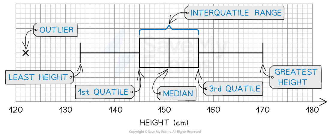
A box plot of this data is as follows:
Box and whisker plot showing height data from a population of girls

The width of the box shows the interquartile range and the overall range is shown by the length of the whiskers
Outliers
Outliers are data points that exist at the extremes above and below the rest of the data
In order for a data point to be categorised as an outlier it needs to be more than 1.5 × the interquartile range above the third quartile or below the first quartile
As shown in the worked example above, the outliers are plotted separately to the whiskers of the plot

Unlock more, it's free!
Was this revision note helpful?
