Practical Skills: Written Assessment (OCR AS Biology)

Exam Questions

3 hours38 questions
1a
Sme Calculator
2 marks

The rate of water loss from a plant shoot can be measured using a simple potometer, as shown in Figure 1.1 below. The amount of water taken up by the plant shoot can be measured using the scale on the pipette.
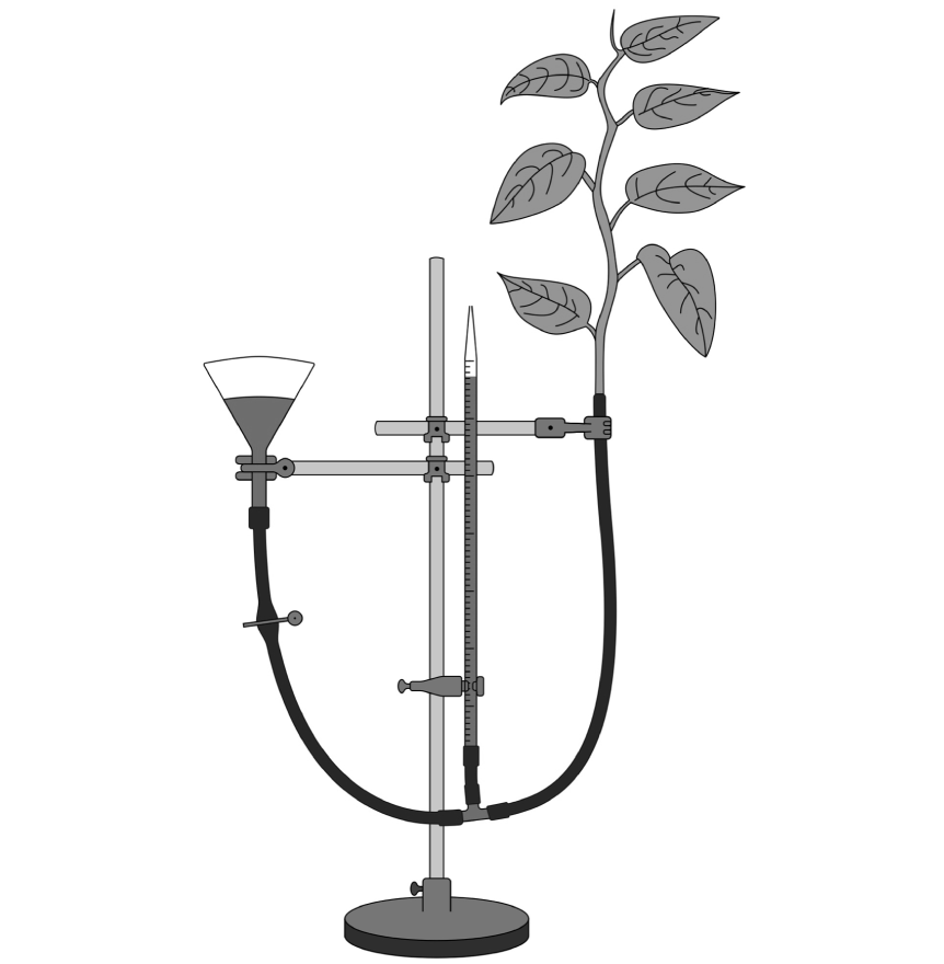
ocr-a-1-1-sqe-q1-potometer 

Figure 1.1

A student used this potometer apparatus and a lamp to investigate the effects of light intensity on the rate of water loss from the plant. They carried out the experiment at 5 different light intensities by varying the distance of the lamp from the plant.

Identify the dependent and independent variables in the experiment.

1b
Sme Calculator
2 marks

Describe how the student would measure the rate of water uptake at each light intensity. 

1c
Sme Calculator
3 marks

Identify three variables that must be controlled.

1d
Sme Calculator
1 mark

Describe how the student could ensure that their results are reliable.

Did this page help you?

2a
Sme Calculator
3 marks

A student carried out an experiment to test the effects of temperature on the activity of the enzyme catalase. They used cut cubes of potato and a H2O2 solution, collecting the oxygen released from the reaction in a measuring cylinder with 1 ml graduations. The potato cubes were added to H2O2 solution in water baths at temperatures of 20 ⁰C, 30 ⁰C and 40 ⁰C. A stopwatch was then used to measure oxygen collection in the first minute of the experiment. The experimental setup can be seen in Figure 2.1.

ocr-a-1-1-e-sq-q2-catalase-experiment

Figure 2.1

List three variables that must be controlled in this experiment. 

2b
Sme Calculator
2 marks

Using the description and Figure 2.1 above, identify two potential sources of error in this experiment. 

2c
Sme Calculator
4 marks

At 30 ⁰C, the student recorded a mean of 20 ml of oxygen in the first minute across 3 repeats of the experiment. 

(i)
State the uncertainty value introduced by the measuring cylinder.

[1]

(ii)
Calculate the percentage error introduced by the measuring cylinder. 

   [2]

(iii)
Describe one way in the student could have improved the accuracy of the measurement.

[1]


Did this page help you?

3a
Sme Calculator
6 marks

A student wanted to investigate the frequency of two flowering plant species, cowslip and oxeye daisies, in two areas of meadow using a quadrat. She carried out 10 samples in each meadow. The results are displayed in Table 1 below

Table 1

  Meadow 1 Meadow 2
Sample no. Cowslip (n) Oxeye daisy (n) Cowslip (n) Oxeye daisy (n)
1 3 5 4 5
2 4 7 1 9
3 3 8 2 8
4 1 5 2 5
5 5 7 3 2
6 1 6 1 7
7 3 7 4 5
8 6 1 2 1
9 2 3 3 5
10 3 7 1 4
Mean:        


The student wanted to compare the data she had collected from each meadow.

(i)
Calculate the mean value of each of the data sets (to the nearest whole number).
[2]
(ii)
State whether the data in Table 1 above is qualitative or quantitative.
[1]
(ii)
Identify the best type of graphical format for the data in Table 1 above
[1]
(iv)
The student draws a graph of her results.
Identify the labels on the x- and y-axis.
[2]
3b
Sme Calculator
4 marks

The student concluded that the oxeye daisy had a higher frequency than the cowslip. She wanted to improve her data set to ensure that her conclusions were valid.

(i)
In order for her sample to be representative, it was important that her sample sites were selected randomly and were not selected in a way that prioritised certain areas in the meadow. Describe how the student could ensure that her sample site selection was random.

[2]

(ii)

Describe one way by which the student could ensure that her results were not anomalous.

[1]

(iii)

The student wanted to analyse whether there was a significant difference between the frequencies of the two flower species.

State one way in which she could achieve that.

[1]

Did this page help you?

4a
Sme Calculator
6 marks

A group of scientists wanted to test whether a new blood-pressure medication was effective. They carried out an experiment on 20 patients who had blood pressure that was higher than normal (Drug group). They tested the patients’ resting blood pressure before giving them the medication, and again after they had been on regular doses of the medication for 1 month. They carried out the same test on another 10 patients using a placebo (Placebo group). The results are displayed in Table 1 below.

Table 1


Initial Blood Pressure (mmHg)

(+/- standard deviation)


Blood Pressure after 1 month (mmHg)

(+/- standard deviation)

  Systolic Diastolic Systolic DIastolic
Placebo 120 (+/- 7) 70 (+/- 8) 118 (+/- 6) 67 (+/- 7)
Drug 140 (+/- 6) 100 (+/- 7) 130 (+/- 5) 90 (+/- 7)

The scientists examined the data in Table 1 above

(i)
Calculate the difference in average systolic blood pressure before and after the medication in the Placebo group. 
[1]
(ii)
Calculate the differences in average systolic blood pressure before and after the medication in the Drug group.
[1]
(iii)
State the range of values included in the standard deviation of the Systolic blood pressure before the medication and after the medication in the Placebo group.
[2]
(iv)
State the range of values included in the standard deviation of the Systolic blood pressure before the medication and after the medication in the Drug group.
[2]
4b
Sme Calculator
2 marks

Based on your answers to a(iii) and (iv), state whether there is a significant difference in the systolic blood pressure of the placebo group in comparison to the systolic blood pressure of the drug group.

Explain your answer.

4c
Sme Calculator
3 marks

Suggest three ways in which the scientists could improve this study.

Did this page help you?

5a
Sme Calculator
4 marks

Using appropriate units when making calculations and analysing experimental results is important. 

A species of flowering plant requires a space with the dimensions 10 cm by 10 cm to grow. A plant scientist wanted to work out how many plants could fit in an experimental plot with a surface area of 100 m2.
 

(i)
Calculate the surface area of the plant’s required growing area in m2.
[2]

(ii)
Use your answer from (a)(i) to calculate the number of plants that can be grown in the experimental plot.
[2]
5b
Sme Calculator
5 marks

A student compares how much oxygen gas is produced from photosynthesis in two species (Species A and B) of aquatic plant. 

The Species A produces 10 cm3 in 300 seconds

The Species B produces 0.000005 m3 in two minutes

(i)
Calculate the rate of oxygen production of Species A and Species B in cm3 per minute.

[4]

(ii)
Use your answer from (b)(i) to calculate the difference in the rate of oxygen production between Species A and Species B.
[1]

Did this page help you?

1a
Sme Calculator
5 marks
(a)
A student carried out an investigation into the effect of ethanol on the permeability of cell membranes in beetroot.

The student’s method comprised the following five steps:

  1. Cut equal sized pieces of beetroot using a cork borer.
  2. Wash the pieces in running water.
  3. Place the pieces in 100cm3 of different concentrations of ethanol.
  4. After 5 minutes, remove samples from each of the ethanol solutions.
  5. Place each of the samples into a colorimeter to collect quantitative data.

(i)
Each step in the student’s method relies on certain assumptions.

For each assumption listed below, select the numbered step from the student’s method that relies upon that assumption.

Assumption A

                     Pigment will only leak into the solution if membranes are disrupted.

Assumption A relates to step .............

Assumption B

                     Absorbance is proportional to concentration of pigment.

Assumption B relates to step .............

Assumption C

                     Pigment will be released when the beetroot is sliced.

Assumption C relates to step .............

[3]

(ii)
The student kept the ethanol solutions at a constant temperature. State two other variables which need to be controlled in this investigation to ensure the data collected are valid.

[2]

1b
Sme Calculator
5 marks
(b)
Fig. 20.1 shows the graph plotted by the student.

q20b-paper-1-june-2018-ocr-a-level-biology

Fig. 20.1

(i)
Make three criticisms of the way the student has displayed these results.

[3]

(ii)
Explain how carrying out replicates would improve this investigation.

[2]

Did this page help you?

2
Sme Calculator
6 marks

A student investigated the heart rates of smokers and non-smokers.

  • Each test subject had their resting heart rate measured using an electronic heart rate monitor.
  • They ran 1km on a running track and their heart rate after running 500m was recorded.
  • Their heart rate was recorded for a third time 3 minutes after the completion of the exercise.

All test subjects were 18 years old. Subjects were tested between 9am and 4pm on one day, one at a time. Each test lasted approximately 20 minutes in total. The tests were repeated one week later using the same method. Mean heart rates were calculated for each subject.

The student’s plan was to compare the heart rates of smokers and non-smokers using Student’s t-test.

The student’s results are shown in Table 6.

Student Smoker? Gender Resting heart
rate (bpm)
Heart rate
during exercise
Heart rate
after exercise
1 Y Male 60.5 130.0 66.5
2 N Female 67.0 145.5 73
3 Y Male 70.0 120 77.0
4 Y Male 65.5 100 69
5 Y Male 66.0 128.5 75.5
6 Y Female 65.5 115.5 74.5
7 Y Female 73.5 120.5 81
8 N Female 63.0 118 66
9 N Female 71.0 95.5 80.5
10 N Female 65.5 110 71
11 N Male 64.0 145.5 68
12 N Male 52.5 140.0 58.5
13 N Male 54.0 137.5 63
14 N Female 73.0 130.5 81
15 N Female 61.5 124 67
16 N Female 71.0 130 81.5
17 N Male 60.0 122.5 63
18 N Female 64.5 118 69
19 N Female 67.5 130.5 73.5
20 Y Male 72.0 135 82
21 Y Female 69.5 110  75.5

Table 6

Suggest and explain improvements that the student could make to his experimental method and his presentation of data.

In your answer you should explain the benefits of your suggested improvements.

[6]

Did this page help you?

3a
Sme Calculator
5 marks
(a)

Water moves by osmosis in living organisms.

(i)
Define osmosis.
[2]
(ii)
Plants rely on osmosis for support.

Explain the importance of osmosis in plant support.
[3]
3b
Sme Calculator
4 marks
(b)
The apparatus shown in Fig. 16 can be used to demonstrate osmosis.

q16b-paper-2-june-2019-ocr-a-level-biology

Fig. 16

When the capillary tube with visking tubing bag was placed in solution Y, the level of solution X inside the capillary tube rose from 10.5mm to 26.5mm.

(i)
The ruler used to measure the distance along the capillary tube was accurate to the nearest 0.5mm.

Calculate the percentage uncertainty of the measurement.

uncertainty = ............................. % [2]

(ii)
What conclusions can be drawn about the composition of solutions X and Y?

[2]

3c
Sme Calculator
7 marks
(c)
A group of students used the following method to investigate osmosis in plant cells.

  • Cut pieces of plant material of equal surface area ensuring no skin is present.
  • Rinse to remove cell debris.
  • Gently pat the plant pieces dry with a paper towel.
  • Weigh each piece and record mass.
  • Put the plant piece in a 200cm3 beaker.
  • Cover plant piece with 50cm3 of sucrose solution.
  • Use sucrose solutions of 0, 0.1, 0.3, 0.5, 0.7moldm–3.
  • Leave for 24h.
  • Remove the piece of plant material.
  • Dry carefully using a paper towel.
  • Weigh the plant piece and record the mass.
  • Calculate the percentage change in mass for each piece.
  • Repeat twice for each sucrose concentration.

The students investigated material from three different plants: carrot, courgette and potato.
Their results are shown in Table 16.

Plant Sucrose
concentration /
mol dm-3
Percentage change in mass
Replicate 1 Replicate 2 Replicate 3 Mean

Carrot

0 + 6.0 + 5.8 + 5.8 + 5.87
0.1 + 4.2 + 4.1 + 4.3 + 4.20
0.3 + 1.5 + 1.5 + 1.3 + 1.43
0.5 - 2.4 - 2.3 - 2.1 - 2.27
0.7 - 6.3 - 6.1 - 6.3 - 6.23

Courgette

0 + 7.9 + 7.8 + 7.6 + 7.7
0.1 + 5.5 + 5.5 + 5.5 + 5.50
0.3 + 1.9 + 1.8 + 2.0 + 1.90
0.5 - 1.2 - 1.4 - 1.1 - 1.23
0.7 - 4.3 - 4.4 - 4.1 - 4.27

Potato

0 + 5.7 + 5.8 + 5.7 + 5.77
0.1 + 3.1 + 2.9 + 3.0 + 3.00
0.3 - 0.3 - 0.4 - 6.0 - 0.43
0.5 - 2.4 - 2.2 - 2.5 - 2.37
0.7 - 6.1 - 5.9 - 5.1 - 5.70

Table 16

(i)
Explain why it was necessary to calculate percentage change in mass.
[2]
(ii)
The students identified replicate 3 of the potato in 0.7moldm–3 sucrose as anomalous.

Suggest a practical error by the students that might have caused this result to be anomalous and explain the likely effect of this error.
[2]
(iii)
Use Table 16 to identify which plant cells contained the highest concentration of sucrose.

Justify your conclusion.
[3]

Did this page help you?

4
Sme Calculator
3 marks
(a)
Fig. 2.3 shows the relationship between body mass and lifespan in a range of mammal species.q2c-paper-3-june-2019-ocr-a-level-biology
Fig. 2.3
(i)
Describe the relationship between body mass and lifespan shown in Fig. 2.3.

 [1]

(ii)
What conclusion can you draw from Fig. 2.3 about the lifespan of naked mole rats in comparison to other mammals?
 [1]

Did this page help you?

5a
Sme Calculator
8 marks
(a)
Fig. 16 shows pressure changes during the cardiac cycle.


q16a-paper-1-june-2019-ocr-a-level-biology
Fig. 16

(i)

Using Fig. 16, compare the changes in pressure in the left ventricle with the changes in pressure in the left atrium.
[4]
(ii)
Using Fig. 16, calculate the heart rate of this individual.

Give your answer to 2 significant figures.
heart rate = .......................................................... [1]

(iii)
Using Fig. 16, calculate the percentage change between minimum and maximum pressure in the aorta.

Give your answer to 2 significant figures.
percentage change = .......................................................... [2]

(iv)
Name the valve which closes at point X on Fig. 16.
 [1]
5b
Sme Calculator
3 marks
(b)
The heart supplies oxygenated blood to the tissues.

VO2max is a measurement of the maximum volume of oxygen that an individual can use during intense exercise in a given time.

Smart watches can estimate the VO2max of an individual by measuring heart rate while exercising.

Having a higher VO2max is associated with improved aerobic fitness.

Two male students exercised for 30 min and used smart watches to record their VO2max.
Table 16 shows their masses and the VO2max values they recorded.

Student Mass (kg)

VO2max (cm3 kg−1min−1)

1 65 50.4
2 57 48.2

                                       Table 16

Student 1 drew the following conclusion from this result:

q16b-paper-1-june-2019-ocr-a-level-biologyStudent 2 said that this conclusion is invalid because several variables have not been controlled.

State three variables necessary for a valid comparison that have not been controlled in the above experiment.
[3]

Did this page help you?

6
Sme Calculator
8 marks

The Madidi National Park, in the South American rainforest, is home to a wide variety of species.
The largest predator in the area is the jaguar. These large cats are well camouflaged and hunt mostly at night. A single individual can cover a very large area.

(a)
In 2007 the Wildlife Conservation Society (WCS) attempted to estimate the population of jaguars in the Madidi National Park.

  • Digital camera traps were placed in areas that jaguars were likely to visit.
  • If an infrared beam was broken by an animal, the camera was activated.
  • The camera then took a photograph of the animal.

(i)
Suggest why it was not appropriate to estimate the number of jaguars using the capture-recapture technique.
 [2]
(ii)
Most studies estimate the population density of jaguars in the South American rainforest to be 5 individuals per 100km2.

In the 2007 study:
  • 100 camera traps were set up covering an area of 271km2.
  • 28 images of 9 different jaguars were recorded.
How well do these results support a population estimate of 5 individuals per 100km2?

 [4]

(iii)
Other evidence used to estimate the jaguar population includes footprints and reports of sightings by local humans.

Suggest one disadvantage of each of these methods for estimating the size of the jaguar population.

human sightings .....................................
footprints ....................................................

[2]

Did this page help you?

7a
Sme Calculator
2 marks

The potato plant, Solanum tuberosum, is a staple food plant in many parts of the world.

Potatoes are susceptible to infection by a pathogen called Phytophthora infestans, which causes a disease known as potato late blight. The most visible sign of the disease is a brown discolouration of the leaves.

Some varieties of potato are resistant to infection by P. infestans.

(a)
State two ways in which an individual S. tuberosum plant could respond to infection by P. infestans.

[2]

7b
Sme Calculator
1 mark
(b)
The resistance of different varieties of S. tuberosum to infection by P. infestans was investigated.

  • Three different clones, A, B and C, of S. tuberosum were used.
  • The clones were grown in adjacent fields over the same time period.
  • The percentage of leaf area affected by the disease was estimated at regular intervals.
The results are shown in Fig. 18.q18b-paper-2-june-2017-ocr-a-level-biology


Fig. 18

(i)
Suggest why it is important to use clones in an investigation such as this.
 [2]

(ii)
State how a clone of potatoes could be produced for this investigation and explain why it is important to carry out this procedure under aseptic conditions.

procedure .........................................................................
asepsis is important because ...........................................
 [2]

(iii)
The extent of infection is estimated by comparing the area under the curve from the graph. The area under the curve for clone B is 1250. (Units can be ignored in this instance.)

 
Using Fig. 18, calculate the approximate area under the curve, between day 35 and day 98, for clone C.

[3]

(iv)
Calculate the area under the curve for clone C as a proportion of the area under the curve for clone B.

 [1]

(v)
Using Fig. 18, suggest why the area under the curve is used as a measure of infection rather than the area of leaf that is visibly affected on a given day.
 [2]

(vi)
The clones were planted in adjacent fields in order to control variables such as temperature, wind speed and rainfall.

Suggest two other abiotic variables that this precaution was intended to control.
[2]

Did this page help you?

8a
Sme Calculator
3 marks

The effect of wave action on the height of the shells of the dog whelk (Nucella lapillus) was investigated by comparing an exposed shore and a sheltered shore.

q3-paper-3-specimen-ocr-a-level-biology

  • A random sampling technique was used to collect 50 shells from an exposed shore.
  • The shell height was measured from the base to the conical tip. The whelk was returned to its location.
  • The process was repeated for the sheltered shore.
  • All the results were recorded in Table 3.1.
Location Height of shell (mm) Range Mean SD
Sheltered
shore
26 28 27 26 28 23 28 23 26 28  
29 29 29 29 29 28 29 29 29 29
30 31 30 29 32 29 30 29 30 32
33 35 34 32 35 32 34 32 33 35
37 39 38 37 39 35 38 36 37 39 16 31.3 4.1
Exposed
shore
15 17 16 15 23 15 23 16 13 15  
17 24 18 17 17 14 17 18 16 17
19 19 20 24 18 20 19 20 18 20
23 14 24 14 21 20 23 17 21 23
25 25 28 26 25 27 25 28 25 27 15 20.0 4.2

Table 3.1

(a)

The t test can be used to determine the significance of the differences between shell height on the exposed shore and the sheltered shore.

(i)

Calculate the t value for the data using the formula:

t space equals space fraction numerator open vertical bar stack x subscript 1 with bar on top space minus space top enclose x subscript 2 end enclose close vertical bar over denominator square root of open parentheses fraction numerator s subscript 1 superscript 2 over denominator n subscript 1 end fraction plus space fraction numerator s subscript 2 superscript 2 over denominator n subscript 2 end fraction close parentheses end root end fraction

where,

open vertical bar stack x subscript 1 with bar on top space minus space top enclose x subscript 2 end enclose close vertical bar is the difference in mean values of sample 1 and sample 2

s subscript 1 superscript 2 and s subscript 2 superscript 2are the squares of the standard deviations of the samples

n1 and n2 are the sample sizes.

Give your answer to two decimal places.

 [2]

(ii)

The null hypothesis is that there is no difference between the means of the two shell populations.

The critical values at 98 degrees of freedom are shown in Table 3.2.

Degrees of freedom p = 0.10 p = 0.05 p = 0.01 p = 0.001
98 1.67 2.00 2.64 3.41

Table 3.2

Using the table of critical values, explain whether the student would be able to accept or reject the null hypothesis as a result of the t value you calculated in part (i).

[1]

8b
Sme Calculator
4 marks
(b)
The students organised the data from Table 3.1 into classes.

The organised data is shown in Table 3.3.

Sheltered shore Exposed shore
Height (mm) Tally Total Height (mm) Tally Total
23–26 straight I up diagonal strike III 5 11–14 IIII 4
27–30 straight I up diagonal strike III space straight I up diagonal strike III space straight I up diagonal strike III space straight I up diagonal strike III space space II 22 15–18 straight I up diagonal strike III space II end strike 7
31–34 straight I up diagonal strike III space straight I up diagonal strike III space straight I 11 19–22 straight I up diagonal strike III space straight I up diagonal strike III space II 12
35–38 straight I up diagonal strike III space IIII 9 23–26 straight I up diagonal strike III space straight I up diagonal strike III space II 12
39–42 III 3 27–30 IIII 4

Plot the most suitable graph of the data given in Table 3.3.

q3b-paper-3-specimen-ocr-a-level-biology

[4]

8c
Sme Calculator
3 marks
(c)
Use the data and graph to discuss any correlation between the height of the whelk shell and the type of shore.

Suggest explanations for your findings.
[3]
8d
Sme Calculator
2 marks
(d)
Suggest a limitation of the procedure used to gather the data in this experiment and recommend how you could improve this.
[2]
8e
Sme Calculator
1 mark
(e)
How could the students improve the accuracy of their data?
[1]
8f
Sme Calculator
3 marks
(f)
Discuss the validity of the conclusions you have made during this experiment.
[3]

Did this page help you?

1a
Sme Calculator
5 marks

A student wanted to investigate how length of day period affects the rate of plant growth. She decided to use common bean plants and set up her experiment in a room in the school laboratory. 

Explain how the student could carry out her experiment in the laboratory. Give details of how she could collect data.

1b
Sme Calculator
6 marks

List three control variables in this experiment AND explain how each could be controlled. 

1c
Sme Calculator
1 mark

Suggest the most appropriate way to present the data.

Did this page help you?

2a
Sme Calculator
4 marks

Two students wanted to test the effects of light intensity on the rate of photosynthesis in pond weed. 

Student 1 used the setup in Figure 2.1, while Student 2 used the setup in Figure 2.2. 

ocr-a-1-1-h-sq2-fig-1-photosynthesis

Figure 2.1ocr-a-1-1-h-sq2-fig-2-photosynthesis

Figure 2.2

Compare how the two experimental setups would affect the validity and accuracy of the results. Give reasons for your answers.

2b
Sme Calculator
4 marks
(i)
Each student also used a stopwatch in their experiment. Explain what data each student would collect from each experiment.

[2]

(ii)
Describe the relationship each student should expect to observe in their data.

[2]

2c
Sme Calculator
3 marks

Suggest how the students could adapt the experiment to test the effects of temperature on photosynthesis.

Did this page help you?

3a
Sme Calculator
3 marks

A student wanted to use a 0.5 m x 0.5 m quadrat to carry out a line transect up a 300 m stretch of shore perpendicularly to the water line. They carried out quadrats every 5 metres along the transect.

Calculate the total area covered by the transect quadrats in cm2.

3b
Sme Calculator
6 marks

A student investigated the effects of surface area on osmosis in different sized potato cubes. They cut sets of cubes of the following sizes:

  • 1 cm3
  • Sides of 5 mm each
  • Sides of 0.25 cm each

They then weighed equal masses of each cube size and put them in different sugar solutions for 10 minutes. They then removed the cubes from the solution, dabbed off the excess moisture with tissue paper and weighed each set of cubes. 

(i)
Calculate how many times larger the 1 cm3 cubes were than the 0.25 cm.
[2]
(ii)
The student used a ruler with 1 mm graduations to cut the cubes.
Calculate the percentage error of the measurement along one edge for each cube size. 

[3]

(iii)
Suggest which set of cubes would show the greatest increase in mass in a hypotonic solution, given equal masses of each cube size were used.
[1]

Did this page help you?

4a
Sme Calculator
2 marks

In a clinical trial for a new drug affecting insulin sensitivity, 20 subjects were given 100 mg tablets of either the drug or a placebo. Subjects’ blood glucose response was tested before and after the medication. 

Calculate how many tablets would be needed to provide a drug dose of 5 mg per kilo for an 80 kg man. 

4b
Sme Calculator
5 marks

The scientists found that this dose was too low to produce a significant effect. In a previous experiment 1000 mg was found to be effective but created too many side effects. 

Design an experiment to test what the lowest effective dose would be. Include the variables that should be controlled.

4c
Sme Calculator
5 marks

The glucose monitors used to measure subjects’ insulin responses had a percentage error of 6%. 

(i)
Using this information and the information given at part (a), evaluate the reliability of the conclusions that could be drawn about the appropriate drug dosage from the experimental data. 

[3]

(ii)
Suggest how the reliability of the experiment could be improved.
[2]

Did this page help you?

5a
Sme Calculator
4 marks

An ecologist wanted to study the change in arthropod species in a 100 m x 100 m woodland over the course of 5 years. Each year, they conducted sweep-net samples and pitfall trap samples and recorded the mean abundance of 4 key species across 10 randomly-selected 1 m2 sample sites. Their results are presented in Table 1 below.

Table 1

  Year 1 Year 2 Year 3 Year 4 Year 5
Wood white butterfly 3 3 1 2 1
Earwig  5 2 2 2 1
Cockchafer beetle 3 2 1 0 0
Midge  6 6 7 6 25

Explain the measures the ecologist could take to ensure that their data was valid.

5b
Sme Calculator
3 marks

Describe the trends that can be observed in the data over time.

5c
Sme Calculator
4 marks

The ecologist wanted to use their data to understand changes in species abundance over the whole study site.

(i)

Describe how the ecologist would calculate changes in the abundance of these species
over time in the whole study area.

[2]

(ii)
Describe the most useful way for the ecologist to display this data.
[2]

Did this page help you?