Coupled First Order Linear Equations (Edexcel A Level Further Maths: Core Pure)

Revision Note

Roger

Author

Roger

Last updated

Coupled First Order Linear Equations

What are coupled first order linear differential equations?

  • Coupled first order linear differential equations are a pair of simultaneous differential equations of the form

table attributes columnalign right center left columnspacing 0px end attributes row cell fraction numerator d x over denominator d t end fraction end cell equals cell a x plus b y plus straight f left parenthesis t right parenthesis end cell row cell fraction numerator d y over denominator d t end fraction end cell equals cell c x plus d y plus straight g left parenthesis t right parenthesis end cell end table

    • a, b, c and d are real constants
    • f(t) and g(t) are functions of t
      • In your exam these functions will usually be either zero or else simply equal to a constant
    • The equations are described as ‘coupled’ because the rate of change of each of the variables depends not only on the variable itself but also on the other variable
  • Systems of coupled differential equations often occur in modelling contexts where two variables are expected to interact
    • For example x may refer to the size of a population of prey animals, and y to the size of a population of predators
      • We would expect the rate of change of the prey animal population to depend on the number of prey animals there are to reproduce, but also on the number of predator animals eating the prey animals
      • Similarly we would expect the rate of change of the predator animal population to depend on the number of predator animals there are to reproduce, but also on the number of prey animals there are for the predators to eat

How do I solve coupled first order linear differential equations?

  • You can solve coupled systems by turning them into an uncoupled second order differential equation that you know how to solve
    • For example, consider the coupled system
    • fraction numerator d x over denominator d t end fraction equals 0.6 x plus 2 y
fraction numerator d y over denominator d t end fraction equals 3.12 x plus 0.4 y
  • STEP 1Rearrange one of the equations to make the variable that is not in the derivative the subject
    • We can rearrange the first equation to get space y equals 0.5 fraction numerator d x over denominator d t end fraction minus 0.3 x
  • STEP 2Differentiate both sides of the equation from Step 1 with respect to t
    • Differentiating gives fraction numerator d y over denominator d t end fraction equals 0.5 fraction numerator d squared x over denominator d t squared end fraction minus 0.3 fraction numerator d x over denominator d t end fraction
  • STEP 3Substitute the equations from Steps 1 and 2 into the coupled differential equation you didn’t use in Step 1
    • Substituting into the second equation gives 

0.5 fraction numerator d squared x over denominator d t squared end fraction minus 0.3 fraction numerator d x over denominator d t end fraction equals 3.12 x plus 0.4 open parentheses 0.5 fraction numerator d x over denominator d t end fraction minus 0.3 x close parentheses
fraction numerator d squared x over denominator d t squared end fraction minus fraction numerator d x over denominator d t end fraction minus 6 x equals 0

    • The result is a second order differential equation in only one of the variables
  • STEP 4Solve the second order differential equation resulting from Step 3
    • Using the standard solution methods for second order differential equations gives the solution 

x equals A straight e to the power of 3 t end exponent plus B straight e to the power of negative 2 t end exponent

  • STEP 5:  To find the solution for the other variable, substitute the solution from Step 4 along with its derivative into the equation from Step 1
    • Differentiate  x equals A straight e to the power of 3 t end exponent plus B straight e to the power of negative 2 t end exponent  to get fraction numerator d x over denominator d t end fraction equals 3 A straight e to the power of 3 t end exponent minus 2 B straight e to the power of negative 2 t end exponent
    • Then substituting into the Step 1 equation gives

space y equals 0.5 open parentheses 3 A straight e to the power of 3 t end exponent minus 2 B straight e to the power of negative 2 t end exponent close parentheses minus 0.3 open parentheses A straight e to the power of 3 t end exponent plus B straight e to the power of negative 2 t end exponent close parentheses
space y equals 1.2 A straight e to the power of 3 t end exponent minus 1.3 B straight e to the power of negative 2 t end exponent

  • STEP 6:  If the question provides initial or boundary conditions you may use these to find the values of A and B, and then go on to interpret your solutions in the context of whatever situation the coupled system of differential equations may be modelling

Worked example

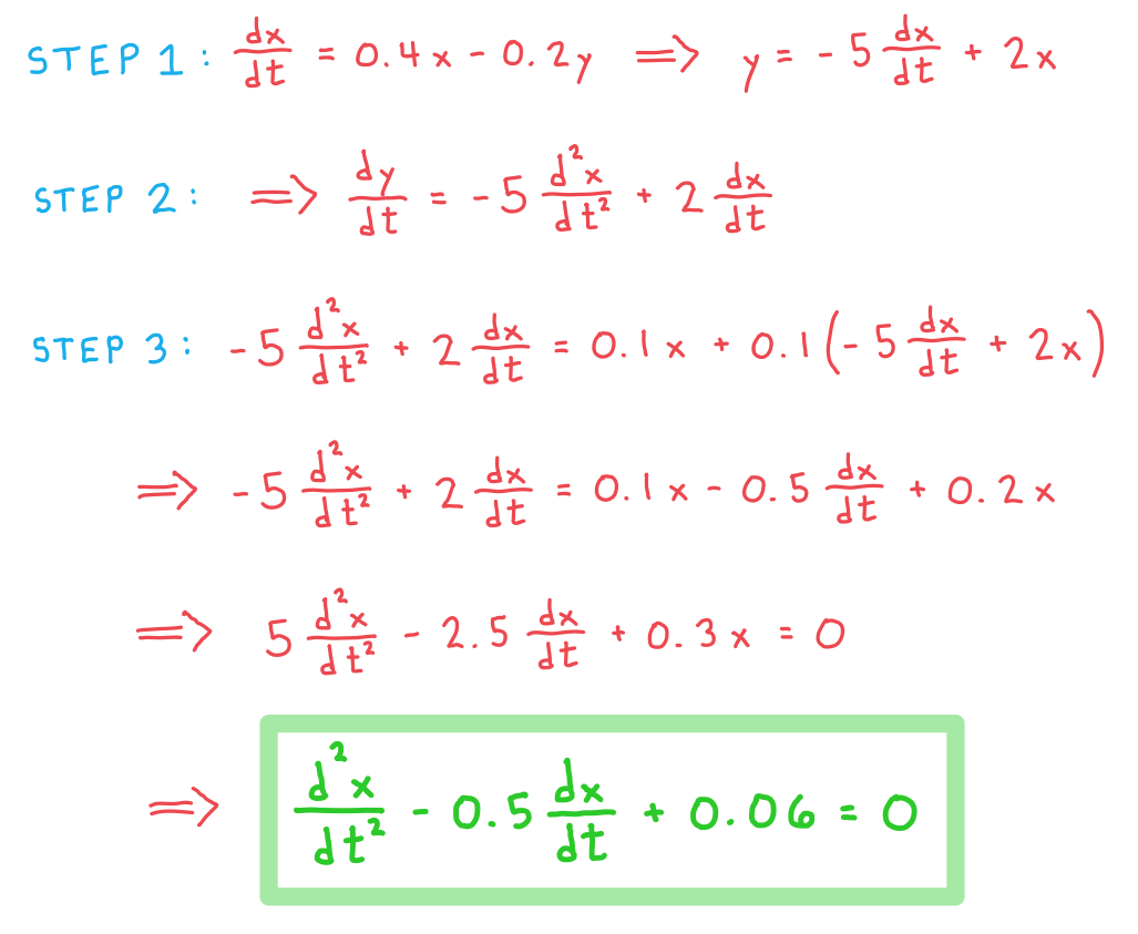
In the following system of coupled differential equations, the variable x represents the population size of a species of prey fish in a particular region of ocean, while the variable y represents the population size of a species of predator fish in the same region.

fraction numerator d x over denominator d t end fraction equals 0.4 x minus 0.2 y
fraction numerator d y over denominator d t end fraction equals 0.1 x plus 0.1 y

a)
Show that fraction numerator d squared x over denominator d t squared end fraction minus 0.5 fraction numerator d x over denominator d t end fraction plus 0.06 x equals 0.

8-2-2-coupled-1st-order-linear-eqns-a-we-solution

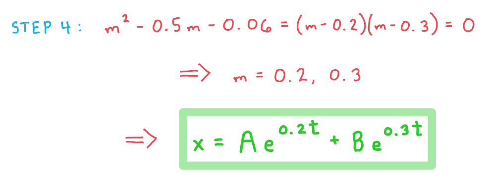
b)
Find the general solution for the number of prey fish in the region at time t.
8-2-2-coupled-1st-order-linear-eqns-b-we-solution

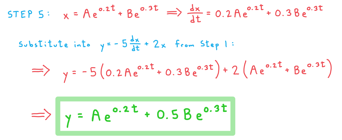
c)
Find the general solution for the number of predator fish in the region at time t.
8-2-2-coupled-1st-order-linear-eqns-c-we-solution

d)
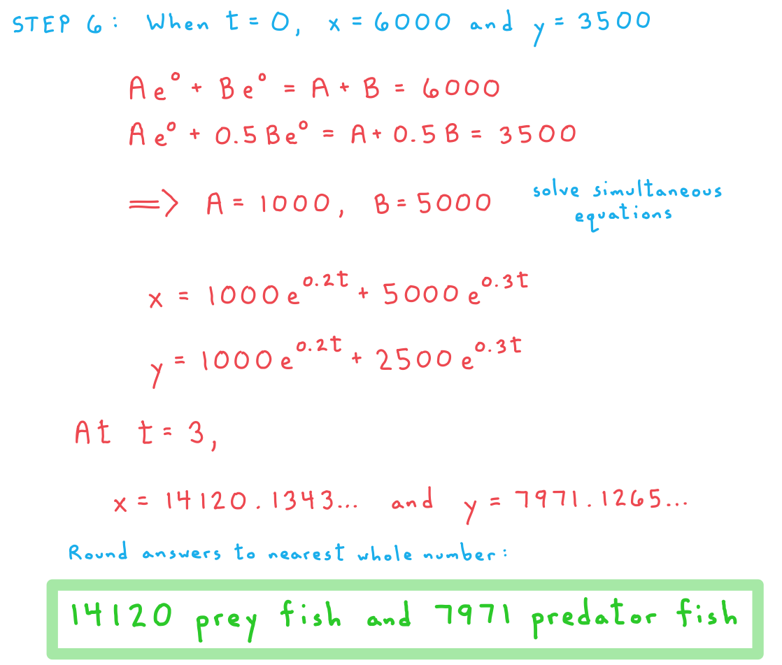
Given that there are initially 6000 prey fish and 3500 predator fish in the region, find the number of each species that the model predicts for time t = 3.
8-2-2-coupled-1st-order-linear-eqns-d-we-solution

e)
Comment on the suitability of the model.
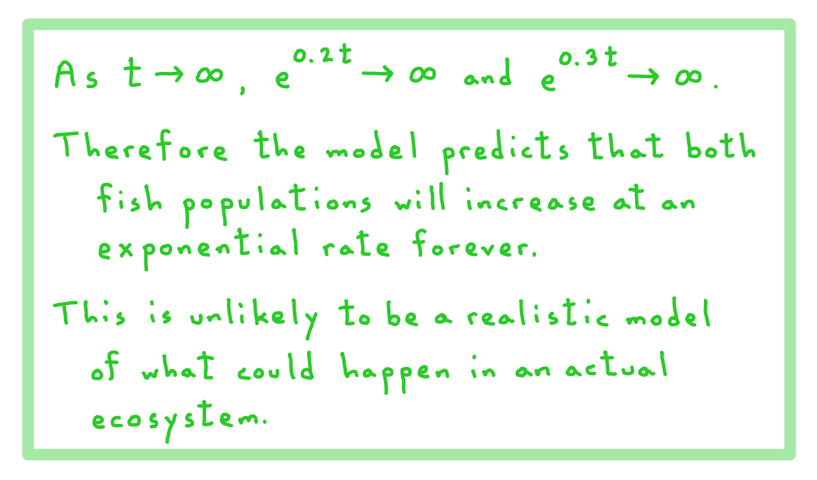
8-2-2-coupled-1st-order-linear-eqns-e-we-solution

You've read 0 of your 5 free revision notes this week

Sign up now. It’s free!

Join the 100,000+ Students that ❤️ Save My Exams

the (exam) results speak for themselves:

Did this page help you?

Roger

Author: Roger

Expertise: Maths

Roger's teaching experience stretches all the way back to 1992, and in that time he has taught students at all levels between Year 7 and university undergraduate. Having conducted and published postgraduate research into the mathematical theory behind quantum computing, he is more than confident in dealing with mathematics at any level the exam boards might throw at you.