Equilibrium Levels of Real National Output (Edexcel A Level Economics A)

Real National Output Equilibrium

Short-run equilibrium

• Real national output equilibrium occurs where aggregate demand intersects with aggregate supply

• According to classical theory, this economy is in short run equilibrium at AP₁Y₁

• Any changes to the components of AD will cause the AD curve to shift left or right creating a new short-run equilibrium

• Any changes to the determinants of SRAS will shift the SRAS curve left or right creating a new short-run equilibrium

Long-run equilibrium

• Classical and Keynesian economists have different views on the long-run equilibrium of real national output

  • Classical economists believe that the economy will always return to its full potential level of output and all that will change in the long-run, is the average price level

  • Keynesian economists believe that the economy can be in long-run equilibrium at any level of output

Diagram analysis

• The LRAS curve demonstrates the maximum possible output of an economy using all of its scarce resources

• The SRAS intersects with AD at the LRAS curve

• This economy is producing at the full employment level of output (Y_FE)

• The average price level at Y_FE is AP₁

Diagram analysis

• The vertical portion of the LRAS curve corresponds to the classical view of LRAS

  • The Keynesian view believes there is a maximum level of possible output

• The LRAS curve becomes elastic at a certain price level as prices cannot fall further

  • Possibly due to minimum wage laws, the existence of trade unions, or long-term employment contracts preventing wage decreases

• Real output national equilibrium can occur at any level of output

  • In this case equilibrium is at the intersection of LRAS and AD (AP₁Y₁)

Changes in the Equilibrium Price Level & Real National Output

Changes using the classical approach

1. An increase in Aggregate Demand (AD)

Diagram analysis

• The initial equilibrium level of output was at AP₁Y₁

• An increase in one of the components of AD (e.g. consumption) causes the AD to increase AD₁→AD₂

• Average prices in the economy rise to AP₂ and the real level of output increases to Y₂

• The new short-run equilibrium is at AP₂Y₂

2. An increase in short run aggregate supply (SRAS)

Diagram analysis

• The initial equilibrium level of output was at AP₁Y₁

  • This equilibrium represents a recessionary or negative output gap equal to Y₁Y_FE

• An increase in one of the determinants of SRAS (e.g. productivity) causes the SRAS to increase SRAS₁→SRAS₂

• Average prices in the economy fall to AP₂ and the real level of output increases to Y₂

• The new short-run equilibrium is at AP₂Y₂

• There is still a negative output gap but it is smaller (Y₂Y_FE)

Changes using the keynesian approach

1. Changes to Aggregate Demand (AD)

Diagram analysis

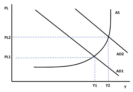
• The economy is initially in equilibrium at the intersection of AD₁ and LRAS

  • The price level is AP₁ and the output is at Y₁

• An increase in any component of AD (e.g. government spending) causes AD to shift from AD₁→AD₂

  • As this increase occurs close to the full employment level of output, there is a large increase in the average price level (AP₁→AP₂), but a relatively small increase in real output (Y₁→Y₂)

• A decrease in any component of AD (e.g. net exports) causes AD to decrease from AD₁→AD₃

  • As this decrease occurs close to the elastic portion of the LRAS curve, there is a relatively larger decrease in the real output (Y₁→Y₃) than the decrease in the average price level (AP₁→AP₃)

• If a further decrease in AD were to take place from AD₃→AD₄, there would be virtually no impact on the average price level, but the real output would fall from Y₃→Y₄

Changes to Long-run Aggregate Supply (LRAS)

1. Changes to LRAS in the Classical Model

• Changes to any of the determinants of LRAS will change the long-run productive potential of the economy

Diagram analysis

• The initial potential output of this economy is seen at Y_FE

  • The economy is in equilibrium at AP₁Y_FE

• A change to the education level in the economy can increase the quality of labour and shift the LRAS to the right from LRAS₁→LRAS₂

  • There is now an increased level of possible output in the economy Y_FE1

• The extra supply in the economy allows prices to fall and output to increase resulting in a new equilibrium at AP₂Y_FE1

2. Changes to LRAS in the Keynesian Model

• As with the Classical model, changes to any of the determinants of LRAS will change the long-run productive potential of the economy

Diagram analysis

• The initial potential output of this economy is seen at Y_FE

  • The economy is in equilibrium at the intersection of AD₁ and LRAS (AP₁Y_FE)

• A change to the immigration policy can increase the quantity of labour and shift the LRAS to the right from LRAS₁→LRAS₂

  • There is now an increased level of possible output in the economy Y_FE1

  • AD is in the vertical portion of the LRAS curve so output will increase (Y_FE→Y_FE1) and average prices will fall (AP₁→AP₃)

• If the starting point of this economy had been the equilibrium at AD₂Y_2, then according to Keynesian thinking, an increase in LRAS would not impact the economy as it is stuck in a depression and requires AD to increase in order to change national output