Variation: t-test Worked Example (OCR A Level Biology)

The ear lengths of two populations of rabbits were measured.

Ear lengths of population A (mm):

62, 60, 59, 61, 60, 58, 59, 60, 57, 56, 59, 58, 60, 59, 57

Ear lengths of population B (mm):

58, 59, 57, 59, 59, 57, 55, 60, 57, 58, 59, 58, 57, 58, 59

Use the t-test to determine whether there is a significant difference in ear length between the two populations.

• Null hypothesis: There is no significant difference between the ear lengths of the rabbits in populations A and B
• Sample sizes:
  • Population A: n₁ = 15
  • Population B: n₂ = 15

Step 1: calculate the mean for each data set:

Mean for population A  x̅₁ = 885 ÷ 15 = 59 mm

Mean for population B  x̅₂ = 870 ÷ 15 = 58 mm

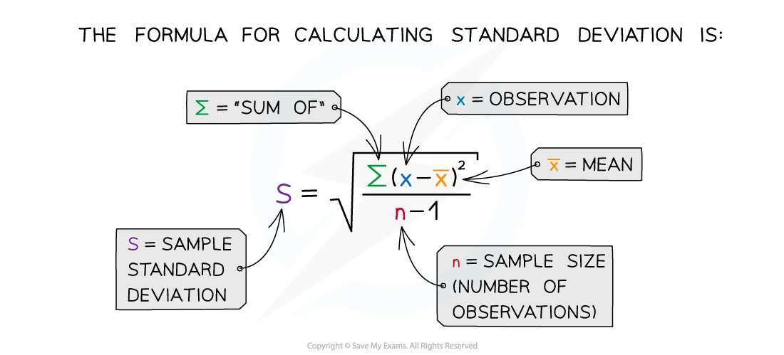
Step 2: calculate the standard deviation (s) for each data set

• Calculate ∑(x - x̄)²

Population A		Population B
Difference between value and mean (x - x̄)	Difference between value and mean squared (x - x̄)2	Difference between value and mean (x - x̄)	Difference between value and mean squared (x - x̄)2
62 - 59 = 3	9	58 - 58 = 0	0
60 - 59 = 1	1	59 - 58 = 1	1
59 - 59 = 0	0	57 - 58 = -1	1
61 - 59 = 2	4	59 - 58 = 1	1
60 - 59 = 1	1	59 - 58 = 1	1
58 - 59 = -1	1	57 - 58 = -1	1
59 - 59 = 0	0	55 - 58 = -3	9
60 - 59 = 1	1	60 - 58 = 2	4
57 - 59 = -2	4	57 - 58 = -1	1
56 - 59 = -3	9	58 - 58 = 0	0
59 - 59 = 0	0	59 - 58 = 1	1
58 - 59 = -1	1	58 - 58 = 0	0
60 - 59 = 1	1	57 - 58 = -1	1
59 - 59 = 0	0	58 - 58 = 0	0
57 - 59 = -2	4	59 - 58 = 1	1
Total ∑(x - x̄)2	36	Total ∑(x - x̄)2	22

• Calculate 

Population A (n1 = 15)	Population B (n2 = 15)
n1 - 1 = 14	n2 - 1 = 14
∑(x - x̄)2 = 36  so 36 ÷ 14 = 2.57	∑(x - x̄)2 = 22  so 22 ÷ 14 = 1.57

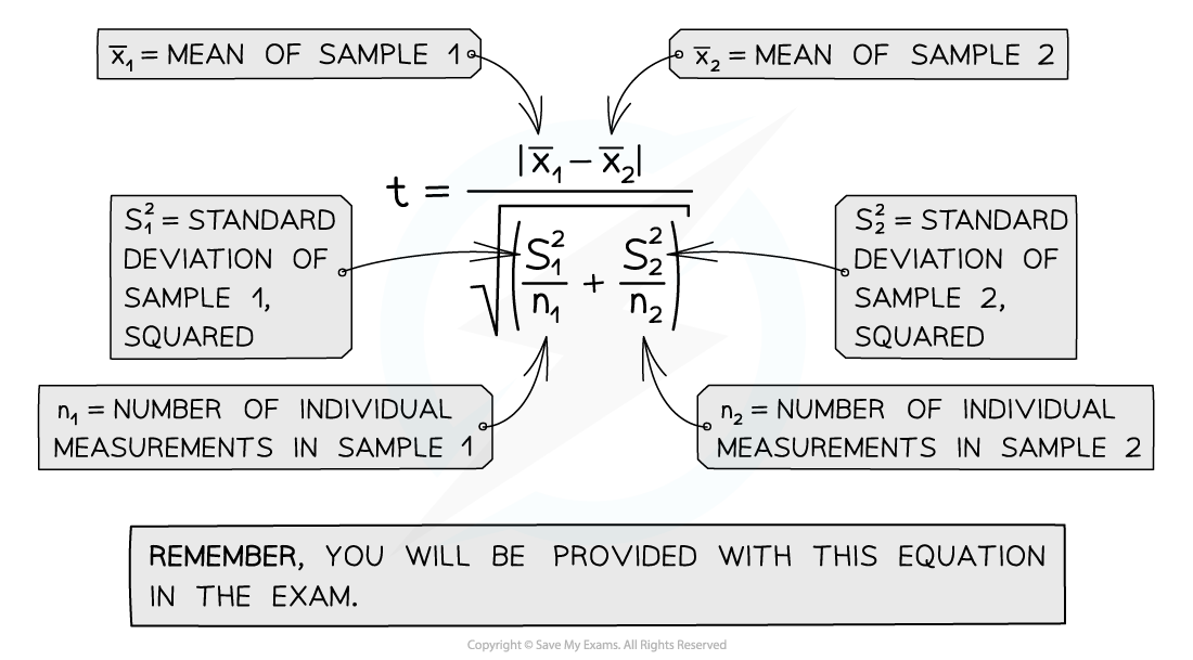
Steps 3-5: use the standard deviations to complete the t test

	Population A	Population B
Mean (x̄)	59	58
Standard deviation (s)	1.60	1.25
Sample size (n)	15	15

Step 6: calculate the degrees of freedom (v) for the data:

v = (n₁ - 1) + (n₂ - 1)

= 14 + 14 

= 28

Step 7: determine where the t value lies in relation to values in a critical values table

Degrees of freedom	Value of t
28	1.70	2.05	2.76	3.67
Probability that chance would have produced this value of t	0.1	0.05	0.01	0.001

• The t value is 1.90, which falls between 1.70 and 2.05 in the critical values table
• In biology we are looking for a less than 5 % probability that any difference between data sets is due to chance, so we are concerned with whether our t valuer is higher or lower than 2.05

Step 8: draw a conclusion

• A conclusion should contain:
  • A reference to the t value, the critical value, the degrees of freedom and the probability level
  • Whether or not there is a significant difference between the means of the two data sets
  • Whether the null hypothesis is accepted or rejected

The t value of 1.90 is less than the critical value of 2.05 at 28 df and a probability level of 0.05

There is no significant difference between the data sets and we can accept the null hypothesis. Any difference between the mean ear lengths of population A and population B is due to chance.