Variation: t-test Worked Example

Worked example

The ear lengths of two populations of rabbits were measured.

Ear lengths of population A (mm):

62, 60, 59, 61, 60, 58, 59, 60, 57, 56, 59, 58, 60, 59, 57

Ear lengths of population B (mm):

58, 59, 57, 59, 59, 57, 55, 60, 57, 58, 59, 58, 57, 58, 59

Use the t-test to determine whether there is a significant difference in ear length between the two populations.

Solution

Null hypothesis: There is no significant difference between the ear lengths of the rabbits in populations A and B
Sample sizes:
- Population A: n₁ = 15
- Population B: n₂ = 15
Step 1: Calculate the mean for each data set:

Mean for population A x̅₁ = 885 ÷ 15 = 59 mm

Mean for population B x̅₂= 870 ÷ 15 = 58 mm

Step 2: Calculate the standard deviation (s) for each set of data

Population A		Population B
Difference between value and mean (x - x̄)	Difference between value and mean (x - x̄)²	Difference between value and mean (x - x̄)	Difference between value and mean (x - x̄)²
62 - 59 = 3	9	58 - 58 = 0	0
60 - 59 = 1	1	59 - 58 = 1	1
59 - 59 = 0	0	57 - 58 = -1	1
61 - 59 = 2	4	59 - 58 = 1	1
60 - 59 = 1	1	59 - 58 = 1	1
58 - 59 = -1	1	57 - 58 = -1	1
59 - 59 = 0	0	55 - 58 = -3	9
60 - 59 = 1	1	60 - 58 = 2	4
57 - 59 = -2	4	57 - 58 = -1	1
56 - 59 = -3	9	58 - 58 = 0	0
59 - 59 = 0	0	59 - 58 = 1	1
58 - 59 = -1	1	58 - 58 = 0	0
60 - 59 = 1	1	57 - 58 = -1	1
59 - 59 = 0	0	58 - 58 = 0	0
57 - 59 = -2	4	59 - 58 = 1	1
Total ∑(x - x̄)²	36	Total ∑(x - x̄)²	22

To find the standard deviations divide the sum of each square by n - 1 for each data set, and take the square root of each value

Population A (n₁ = 15)	Population B (n₂ = 15)
n₁ - 1 = 14	n₂ - 1 = 14
∑(x - x̄)² = 36 so 36 ÷ 14 = 2.57	∑(x - x̄)² = 22 so 36 ÷ 22 = 1.57
$\sqrt{2.57} = 1.60$	$\sqrt{1.57} = 1.25$
$s_{1} = \sqrt{\frac{\sum_{} {(x - \bar{x})}^{2}}{n - 1}} = 1.60$	$s_{2} = \sqrt{\frac{\sum_{} {(x - \bar{x})}^{2}}{n - 1}} = 1.25$

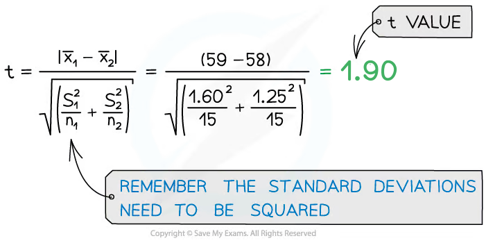
Step 3: Square the standard deviation and divide by n (the number of observations) in each sample, for both samples:

Step 4: Add the values from step 3 together and find the square root

Step 5: Divide the difference between the two means by the value from step 4

Population A	Population B
x̄₁ = 59	x̄₂ = 58
s₁ = 1.60	s₂ = 1.25
n₁ = 15	n₂ = 15

calculation of t value in t test

Step 6: Calculate the degrees of freedom (v) for all the data:

$v = (n_{1} - 1) + (n_{2} - 1) = 14 + 14 = 28$

Step 7: Look at a table that relates t values to the probability that the difference between data sets is due to chance to find where the t value of 1.90 for 28 degrees of freedom (v) calculated lies

Degrees of freedom	Value of t
28	1.70	2.05	2.76	3.67
Probability that chance would have produced this value of t	0.1	0.05	0.01	0.001

Step 8: Draw a conclusion about the statistical relevance of the data

We are considering a confidence level of 0.05, corresponding to a critical value of at least 2.05. However, our t value is 1.90, less than the critical value. So the null hypothesis should be accepted

This means the null hypothesis should be accepted, as there are no significant differences between the two sets of results (any differences between the means of the ear length of rabbits in the two populations are due to chance)

Variation: t-test Worked Example (CIE A Level Biology)

Revision Note

Worked example

Variation: t-test Worked Example

Solution

You've read 0 of your 5 free revision notes this week

Sign up now. It’s free!

Join the 100,000+ Students that ❤️ Save My Exams

Author: Phil